Features:
How We Mapped 1.3m Data Points Using Mapbox
Five things to learn from the Financial Times’ broadband map

A fact of life at the Financial Times is the sheer wealth of cartographic talent here: data visualization editor Alan Smith studied and began his career making maps; visual journalist Chris Campbell crafts some of the FT’s most sumptuous cartographic creations; and interactive design editor Steve Bernard is renowned throughout the interwebs for his encyclopaedic knowledge of QGIS. Accordingly, it was with a combination of excitement and very real dread that, when Alan approached us in late February 2018 to ask if we’d be interested in mapping Britain’s broadband speeds, we said: “Sure! Sounds… great?”
We’d be working with a data set released by the UK’s telecommunications regulator, Ofcom, detailing the speed and availability of broadband internet connectivity for over 1.3m British postcode units. The postcode-level geography presented what would be the first of many challenges in mapping this data: the pricing for the postcode polygons shapefile begins at £26,800 for a limited business license. Pooling our loose change left us some way short of this total, so we went in search of an alternative solution, ultimately deciding on the inverse distance weighting (IDW) interpolation approach detailed in the methodology note of the article.
We set the interpolation process running in QGIS on a Mac Pro and, a mere 11 days later, found ourselves the proud owners of a raster 250m2 grid layer covering the full extent of Great Britain, with the shade of each cell representing the mean download speed of the postcode centroids falling within it. Equipped with the raster and a beautiful red-yellow colour ramp developed by interactive designer Caroline Nevitt, we could start work on the interactive map.
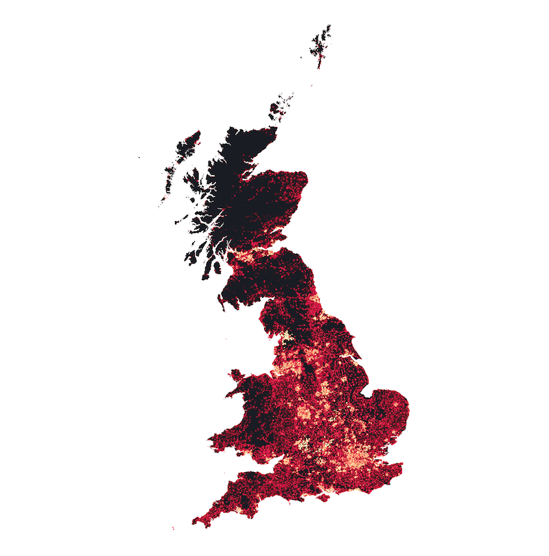
The raster grid layer at country level
We’d used Mapbox GL JS (MGJS) previously for a 3D map of China’s Belt and Road Initiative, which was well received and even found its way onto the Mapbox homepage. We found MGJS fun to work with and, crucially, well documented. Enhancements to the Mapbox Studio web app since then have made it even easier to create and customize data-driven maps.
We’ve increasingly been using React to build interactive pages over the past 18 months, reflecting our team’s move towards a reusable component-centered approach to front-end development. We’d also harbored a desire to use Uber’s suite of WebGL-based visualization tools in a project for some time, and an interactive mapping project of this scale represented an ideal opportunity. Our technology stack was starting to take shape:
- Mapbox GL JS
- React
- react-map-gl (Uber’s React wrapper for MGJS)
This project had an interesting history in that it began as a downtime collaboration between Alan and David and was subsequently elevated to “major project” status following discussions with the FT’s companies editor and telecoms correspondent. An exciting outcome of these was that the findings of Alan’s initial analysis informed and directed some of Nic Fildes’ on-the-ground reporting: for example, he travelled to the B4RN in rural Lancashire after Alan identified the community-run network as having the fastest broadband speeds in Great Britain.
With the companies desk sold on the project, more interactive development and design resources were allocated and discussions began about the most suitable presentation and functionality for the map, a provisional version of which was already in place on a development site. During the design and development process, we experimented with several different user experience (UX) approaches — mostly concerning the map controls — that were ultimately dropped from the published version. Far from being wasted effort, though, these experiments gave us valuable insights into UX for interactive maps that we’re certain to put into practice on future projects.
We also learned plenty through tackling the various unforeseen technical challenges we encountered on this project. Here are just a few of these hard-won nuggets, shared in the hope that they might save fellow interactive mappers some headdesking.
1. Don’t use GeoTIFFs for geometric visualization
Our original plan for the map was to have it display the raster grid layer at lower zoom levels and transition to a vector buildings layer as users zoomed closer to street level. MGJS makes it easy to transition between layers with opacity gradients. We quickly realized, though, that there were issues with the appearance of the grid layer at medium to high zoom levels, at which the cells would begin to artefact and distort into a goopy mess.

The raster grid layer at zoom level 14
The raster, a 4,358px by 5,194px GeoTIFF exported directly from QGIS, simply didn’t have sufficient resolution to provide for sharpness at higher zooms — a limitation that was emphasized by the highly regular geometry of the grid. Fortunately, Mapbox allows GeoTIFF uploads of up to 10GB, so we fired up the command line GIS Swiss Army knife GDAL and made it much, much bigger:
gdal_translate \
  -of GTiff \ # Set output format
  -co BIGTIFF=YES \ # Use BigTIFF variant of TIFF to enable >4GB output file (if necessary)
  -co TILED=YES \ # Pre-cut output image into tiles
  -co BLOCKXSIZE=256 \ # Set output tile width as recommended by Mapbox
  -co BLOCKYSIZE=256 \ # Set output tile height as recommended by Mapbox
  -co COMPRESS=LZW \ # Apply compression as recommended by Mapbox
  -b 1 -b 2 -b 3 \ # Pass only R, G and B bands of input raster (exclude alpha band)
  -outsize 10000% 10000% \ # Scale up horizontally and vertically
  input.tif \ # Input filename
  output-100x.tif # Output filename
The resulting raster was an eye-watering 435,800px by 519,400px and occupied 3.44GB of disk space! The visual integrity of the grid at higher zooms was markedly improved, but we still weren’t convinced by the way it looked at medium zooms.

The raster grid layer at zoom level 9
At these zoom levels, urban areas appeared as largely homogenous, mold-like formations, while more rural areas with sharply contrasting broadband speeds displayed pronounced checkering. Moreover, we felt that we were misrepresenting the data by using 250m2 grid cells, because sparsely populated areas with small numbers of connections — the Welsh valleys, for example (below) — were exaggerated in significance as a consequence of the cell size:

Comparison of the grid layer and buildings layer at zoom level 11
Ultimately, it was the latter concern that led to our decision to drop the grid layer from the map entirely. The buildings layer (below), cropped from the grid layer, provides just as good an overview at lower zoom levels while being arguably more representative of the underlying data.
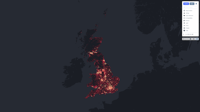
The vector buildings layer at zoom level 5
2. Your GeoJSON can probably be way smaller
At 1.39GB, our buildings layer shapefile greatly exceeded Mapbox’s 260MB shapefile upload limit. The upload limit for GeoJSON is much higher at 1GB, so we set about converting the shapefile using ogr2ogr (also part of the GDAL suite):
ogr2ogr \
  -f geojson \ # Set output format
  -t_srs EPSG:4326 \ # Reproject to Web Mercator
  -select mean \ # Pass required data attributes
  output.json \ # Output filename
  input.shp # Input filename
This resulted in a 3.5GB GeoJSON 😱 We somehow needed to lose 2.5GB from it.
By default, ogr2ogr converts shapefile coordinates to GeoJSON with 15 decimal places of precision. The GeoJSON specification explains that coordinates with a precision of six decimal places are accurate to within approximately 10cm — well beyond what was required for our already simplified buildings layer. We limited our GeoJSON coordinate precision to four decimal places by adding -lco COORDINATE_PRECISION=4 to the above ogr2ogr options. This resulted in a huge reduction in file size — over 40 per cent — but the new GeoJSON still weighed in at more than 2GB.
Each building polygon had an associated (mean) broadband speed value, which had also been calculated to 15 decimal places during the IDW interpolation. For the purposes of our story, one decimal place would be sufficient. Because nothing in GIS is straightforward, attempting to round the values of 2.7m polygons using the field calculator in QGIS invariably resulted in the application crashing, even on a high-end Mac Pro. After several attempts using QGIS 2.16, 2.18 and 3.2, we abandoned the venerable workhorse and instead wrote a small Python script to perform the rounding:
We then re-converted the shapefile with rounded values to GeoJSON. All this, however, was to no avail: the smallest we could make the GeoJSON was 1.8GB — an impressive reduction on the initial 3.5GB but nonetheless unacceptable by Mapbox. We turned instead to Mapbox’s own MBTiles format, of which they permit uploads up to 25GB. Surely that would be enough??
Mapbox also makes available a GeoJSON-to-MBTiles conversion tool called Tippecanoe. This command line tool has a dizzying array of options, including no less than eight different algorithms for dynamically dropping features in order to keep tile sizes under the 500KB limit imposed by Mapbox. We found that dropping the smallest polygons at each zoom level resulted in the least visually jarring behavior when zooming:
tippecanoe \
  -o output.mbtiles \ # Output filename
  -Z0 \ # Minimum zoom level for which to render tiles
  -z16 \ # Maximum zoom level for which to render tiles
  -P \ # Enable parallel processing
  --drop-smallest-as-needed \ # Keep tiles under 500KB by dropping smallest features at each zoom level
  input.json # Input filename
Converting the GeoJSON to MBTiles in this way reduced the upload to an incredible 366MB! Finally, our visualization layer was sitting happily in Mapbox and we were off to the races.
3. Splitting map layers can massively increase the number of visible features
Fresh from our victory over Mapbox’s upload limits, we immediately encountered a drawback to dropping the smallest features at each zoom level: a different subset of features was visible at each zoom level, resulting in some features appearing then disappearing again as the zoom level changed. This opened a new front in our struggle to preserve as much detail as possible at all zoom levels: the 500KB tile size limit.
After a brief period of failing to see the forest for the trees, we remembered that Mapbox supports up to 15 custom layers per map. Could the number of visible polygons be increased by splitting the shapefile and distributing the polygons across multiple layers, thereby reducing the number per layer that would need to be dropped to keep the tile sizes under 500KB?
The answer was a resounding “yes.” We used QGIS’ field calculator again to give each polygon in the shapefile one of nine categories based on its broadband speed value (0–10 mbps, 10–20 mbps etc. up to 80+ mbps). We then split the shapefile using the ‘Split vector layer’ tool. The resultant shapefiles were all converted to GeoJSON then to MBTiles as described above. Perceptibly vibrating with anticipation, we uploaded the new MBTiles to Mapbox and added corresponding layers to the map in Studio. The improvement was striking:
London and surrounding counties

B4RN in North Lancashire
The downside to embedding a map with nine custom layers instead of one, we were to discover, is longer tile loading times. This is particularly noticeable on mobile connections and is something we plan to look into further.
4. Maps aren’t truly responsive by default (but are annoying on mobile by default)
We’d reached the stage at which we had our map, complete with super-detailed visualization layers, embedded in a webpage. It’s all well and good to embed a map and set a fixed initial zoom level for it, but what if that means it’s zoomed in too tight on smaller screens, or that the feature you want to focus on (i.e. Great Britain) is too small on larger ones?
We’ve previously written for Source about the way front-end development works on the FT interactive desk. After scaffolding a new project using our soon-to-be-overhauled Starter Kit, we began exploring ways to make the map zoom to the correct level to fit the whole of Great Britain within the viewport, regardless of the screen size at which the page is loaded.
The solution we settled on was to write a class method called resize() on the map component. resize() first reads the width and height of the map container element using getBoundingClientRect() and passes these values to a new instance of the WebMercatorViewport class from viewport-mercator-project, a utilities library provided by Uber for use with react-map-gl. It then calls the fitBounds() method of WebMercatorViewport, which takes an array of coordinates representing a bounding box (in this case, the southwestern and northeastern bounds of Great Britain) and returns a new viewport object containing a longitude, latitude and zoom level, among other properties. The viewport can then be passed to the interactive map component exported from react-map-gl to configure the map that is ultimately rendered:
resize = () => {
  console.log('Viewport will resize…');

  const width = this.mapContainer.current.getBoundingClientRect().width;
  const height = this.mapContainer.current.getBoundingClientRect().height;
  const viewport = new WebMercatorViewport({ width, height });
  const { zoom, minZoom } = this.props.viewport;
  const bound = viewport.fitBounds(this.props.ukBounds, { padding: 10 });

  if (zoom.toFixed(5) === minZoom.toFixed(5)) {
    this.onViewportChange({
      ...bound,
      minZoom: bound.zoom,
      transitionDuration: 0,
    });
  } else {
    this.onViewportChange({
      width,
      height,
      minZoom: bound.zoom,
    });
  }
};
resize() is called from the componentDidMount() lifecycle method, which fires when a React component is first rendered to the DOM. Calling resize() at this early stage in the component lifecycle ensures that an appropriate minimum zoom level is set for the map on page load. A window resize event listener is also added from componentDidMount(), which calls resize() and updates the map’s minimum zoom level whenever the window is resized (although we used throttle from lodash to ensure that it was called no more than once every 500ms to minimise any performance hit).
componentDidMount() {
  window.addEventListener('resize', throttle(this.resize, 500));
  this.resize();
  this.initialiseMap();
  this.props.getSpeedData();
}
The map would now zoom to perfectly cover Great Britain on load and would adjust this zoom level in response to changes in screen size. Updating the minimum zoom on page resize also meant that users couldn’t zoom out any further than the bounds of Great Britain, regardless of screen size changes. We subsequently added some additional logic to the map component to ensure that the map could not be drag-panned beyond the bounds of Great Britain.
A common criticism of interactive maps (so-called “slippy” maps) is that they have a tendency to capture touch interactions on touchscreen devices, obstructing page scrolling and irritating users in the process. We limited our map to a maximum height of 60 percent of the viewport, leaving plenty of room above and below it for dragging up or down to scroll the page. Additionally, react-map-gl 3.2.9 introduced a touchAction attribute on the interactive map component that can be given the value 'pan-y' to enable vertical page scrolling by dragging up or down on the map itself. [In retrospect, I would have preferred that we didn’t implement this. I think it makes drag-panning the map difficult and confusing on touchscreens, and was largely unnecessary due to the 60 percent viewport height of the map. — David]
5. Performance, particularly on mobile, will need all the help it can get | By Ændrew Rininsland
Redux was added as a way of managing state given there are a lot of ways the user can interact with the page and some components are not children or even siblings of others. We used a fairly normalized store shape as suggested by the Redux docs, which conserves system resources by preventing unnecessary updates to the components. Most of the store updates happen when a map transition occurs, during which quite a number of dispatches occur. We really didn’t explore optimizing this more due to time constraints, but it’s possible there’s more room to improve performance here, for instance by removing the viewport object from the store or by making more efficient use of Mapbox interpolators.
Instead of having a few “container” components that passed state down to their children, often we connected child components directly to the store so we could optimize how state was passed to them (in turn ensuring components would update only when passed relevant state changes). Additionally, given how simple our store was, our reducers could be very generic and contain very little logic, making it pretty trivial to lift state from components to the store.
Our most complex actions were involved when users entered a postcode or used the geolocation functionality, because we did a variety of bounds checking and error handling during these. For these we used redux-thunk, because it’s way simpler than redux-saga or anything else, and our asynchronous state management needs weren’t overly complex (mainly a single fetch request to Amazon S3 and a geolocation API that translated coordinates to postcodes).
Mapbox originally had a few issues when bundling with Webpack. Querying a few folks on News Nerdery, we found that a few had given up entirely and resorted to consuming Mapbox purely via CDN. Because Mapbox is a really big dependency, being able to benefit from Webpack’s dead code removal features ensured we shipped the smallest bundle possible. After a bit of GitHub issue discussion and the creation of a minimalist reproduction, the Mapbox team was able to fix their Browserify config so Mapbox’s web workers no longer caused issues with bundling.
At one point we considered writing an AWS Lambda function to query a table when a user searched for a postcode. In the interests of archivability and performance, instead we separated the CSV table into a JSON file for every row and stored those ~1.56m files on S3, cached by Fastly. This reduced the round-trip latency (admittedly not much of a concern given the size of each data file and the fact that it happens usually no more than once or twice per visit) and meant that we didn’t have to think about managing a Lambda resource post-publication.
We learned so much on this project that this article could easily have been twice or three times its length. We left out topics including:
- how we integrated D3 with React;
- how we settled on the final map controls;
- how we developed a color ramp for use across maps and charts;
- how we approached the display of small multiple maps on mobile devices…
…and many more. Let us know in the comments if you’d like to hear more about these or any of the other topics covered in this article.
The broadband map was a challenging but ultimately hugely rewarding project for our team. We’re excited to take its lessons forward into our next major interactive piece and hope you find them useful too. Happy mapping!
Credits
-
 David Blood
David Blood (@davidcblood) is an interactive news journalist at the Financial Times. His circuitous career path led him through the worlds of film production, business intelligence and communications before reaching journalism in 2014. He joined the FT in 2016 having previously worked with BBC News Labs and the Guardian. His work is focused on interactive visual storytelling and data-driven reporting.
-
 Ændrew Rininsland
Ændrew Rininsland is a developer with the Financial Times interactive graphics team. He is on Twitter, Mastodon and everywhere else as @aendrew.